import pandas as pd
import numpy as np
import requests

from plotnine import ggplot, aes, geom_col, geom_line, labs
from siuba import *
from siuba.dply.forcats import fct_lump
from siuba.siu import callSpace Launches
agencies = pd.read_csv("https://raw.githubusercontent.com/rfordatascience/tidytuesday/master/data/2019/2019-01-15/agencies.csv")
launches = pd.read_csv("https://raw.githubusercontent.com/rfordatascience/tidytuesday/master/data/2019/2019-01-15/launches.csv")
Launches per year
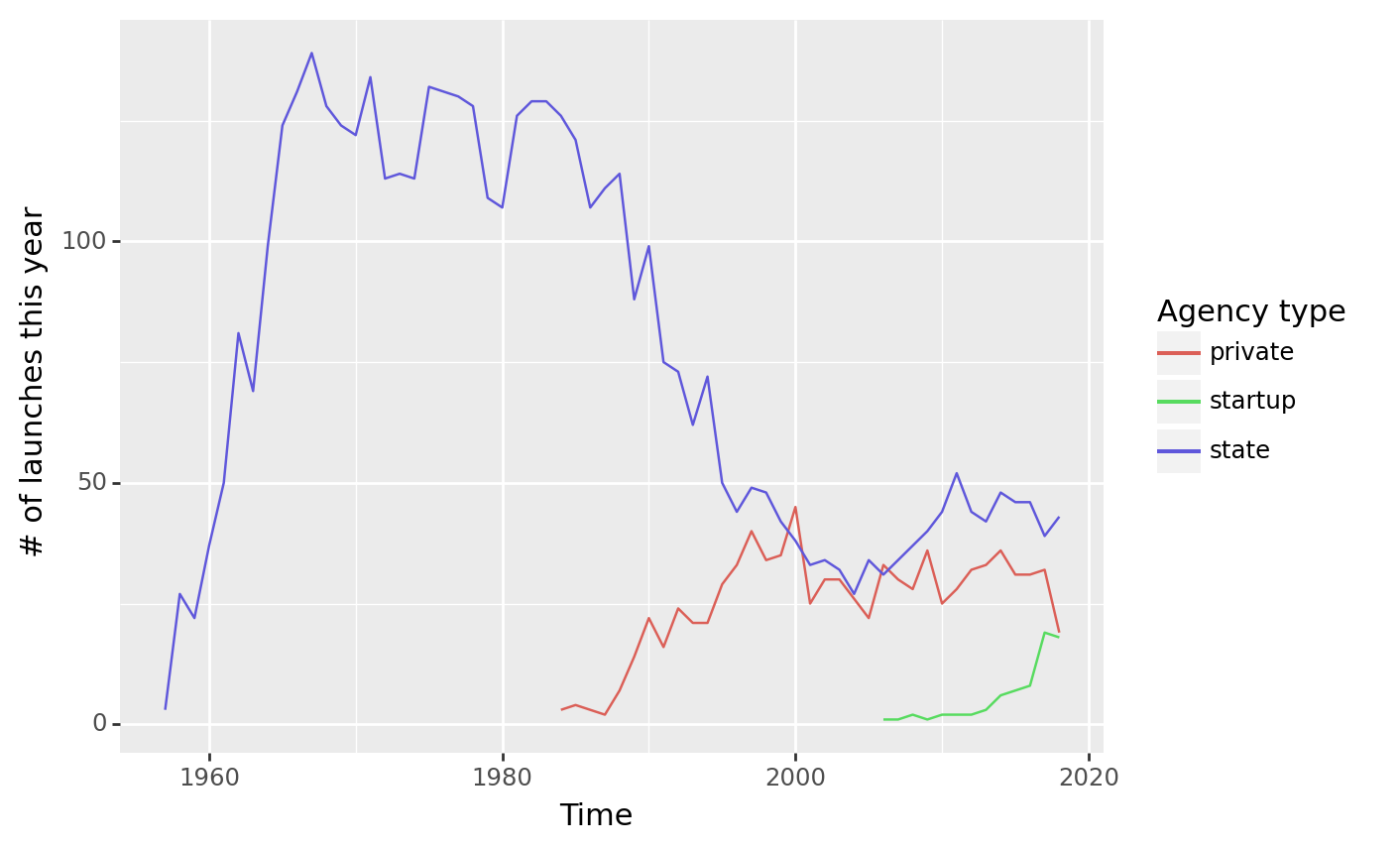
(launches
   >> count(_.launch_year, _.agency_type)
   >> ggplot(aes("launch_year", "n", color = "agency_type"))
    + geom_line()
    + labs(x = "Time", y = "# of launches this year", color = "Agency type")
)
<ggplot: (8770198359007)>Which agencies have the most launches?
In this section, we’ll join launches with agencies, so we can get the agency short names (e.g. SpaceX).
First, though–we want to make sure the column we’re joining on in agencies does not have duplicate values. Otherwise, it will create multiple rows per launch when we join.
agencies >> count(_.agency) >> filter(_.n > 1)| agency | n |
|---|
Now that we know each agencies.agency occurs once, let’s do our join.
agency_launches = launches >> inner_join(_, agencies, "agency")

agency_launches >> count()| n | |
|---|---|
| 0 | 950 |
launches >> count()| n | |
|---|---|
| 0 | 5726 |
Notice that the joined data only has 950 rows, while the original data has almost 6,000. What could be the cause?
To investigate we can do an anti_join, which keeps only the rows in launches which do not match in the join.
launches >> anti_join(_, agencies, "agency") >> count(_.agency, _.agency_type, sort=True)| agency | agency_type | n | |
|---|---|---|---|
| 0 | NaN | state | 2444 |
| 1 | US | state | 1202 |
| 2 | RU | state | 619 |
| 3 | CN | state | 302 |
| 4 | J | state | 78 |
| 5 | IN | state | 65 |
| 6 | I-ESA | state | 13 |
| 7 | F | state | 11 |
| 8 | IL | state | 10 |
| 9 | I | state | 9 |
| 10 | IR | state | 8 |
| 11 | KP | state | 5 |
| 12 | I-ELDO | state | 3 |
| 13 | KR | state | 3 |
| 14 | BR | state | 2 |
| 15 | UK | state | 2 |
Notice that for rows that were dropped in the original join, the agency_type was always "state"!
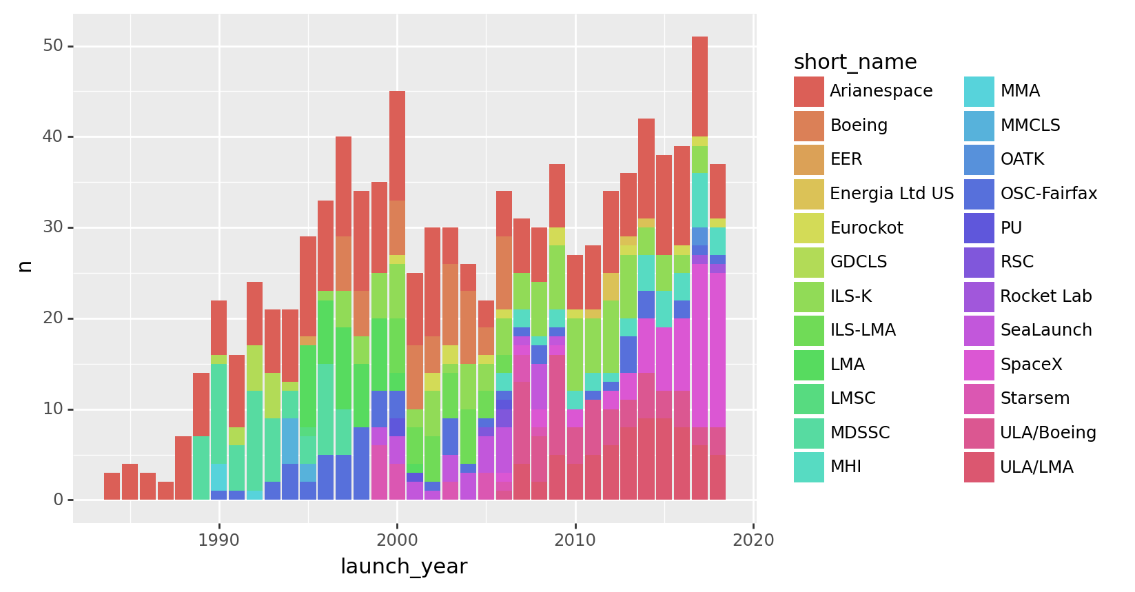
(agency_launches
   >> count(_.launch_year, _.short_name)
   >> ggplot(aes("launch_year", "n", fill = "short_name"))
   + geom_col()
)
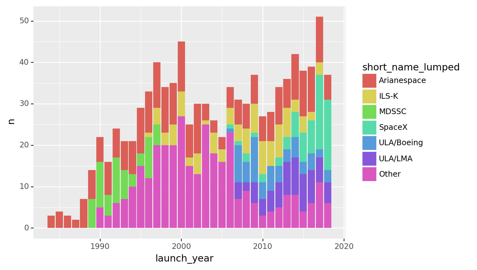
<ggplot: (8770128456732)>(agency_launches
>> mutate(short_name_lumped = fct_lump(_.short_name, n = 6))
>> count(_.launch_year, _.short_name_lumped)
>> ggplot(aes("launch_year", "n", fill = "short_name_lumped"))
+ geom_col()
)
<ggplot: (8770128354094)>Extra: potential improvements
When we joined agencies and launches, columns that had the same names ended up prefixed with _x or _y. We should double check that those columns have identical information, and then drop the duplicate column before joining.
Here’s how you can select just the columns that end with _x or _y:
agency_launches >> select(_.endswith("_x"), _.endswith("_y"))| type_x | state_code_x | agency_type_x | state_code_y | type_y | agency_type_y | |
|---|---|---|---|---|---|---|
| 0 | Ariane 3 | F | private | F | O/LA | private |
| 1 | Ariane 1 | F | private | F | O/LA | private |
| 2 | Ariane 3 | F | private | F | O/LA | private |
| 3 | Ariane 3 | F | private | F | O/LA | private |
| 4 | Ariane 3 | F | private | F | O/LA | private |
| ... | ... | ... | ... | ... | ... | ... |
| 945 | Atlas V 411 | US | private | US | LA | private |
| 946 | Atlas V 541 | US | private | US | LA | private |
| 947 | Atlas V 551 | US | private | US | LA | private |
| 948 | Atlas V 401 | US | private | US | LA | private |
| 949 | Atlas V 551 | US | private | US | LA | private |
950 rows × 6 columns
Extra: parsing big dates in pandas
You might have noticed that this data has a launch_date column, but we only used launch_year. This is because there launch_date has values pandas struggles with: very large dates (e.g. 2918-10-11).
In this section we’ll show two approaches to parsing dates:
- the
.astype("Period[D]")method. - the
pd.to_datetime(...)function.
As you’ll see, the first approach can handle large dates, while the best the second can do is turn them into missing values.
First we’ll grab just the columns we care bout.
launch_dates = launches >> select(_.startswith("launch_"))

launch_dates >> head()| launch_date | launch_year | |
|---|---|---|
| 0 | 1967-06-29 | 1967 |
| 1 | 1967-08-23 | 1967 |
| 2 | 1967-10-11 | 1967 |
| 3 | 1968-05-23 | 1968 |
| 4 | 1968-10-23 | 1968 |
Next we’ll create columns parsing the dates using the two methods.
dates_parsed = (launch_dates
    >> mutate(
        launch_date_per = _.launch_date.astype("Period[D]"),
        launch_date_dt = call(pd.to_datetime, _.launch_date, errors = "coerce")
    )
)

dates_parsed >> filter(_.launch_date_dt.isna()) >> head()| launch_date | launch_year | launch_date_per | launch_date_dt | |
|---|---|---|---|---|
| 547 | NaN | 1962 | NaT | NaT |
| 550 | NaN | 1963 | NaT | NaT |
| 551 | NaN | 1963 | NaT | NaT |
| 1012 | 2918-10-11 | 2018 | 2918-10-11 | NaT |
| 1160 | NaN | 2012 | NaT | NaT |
Notice that one of the years was 2018, but it was miscoded as 2918 in 2918-10-11.
Notice that it is..
- an
NaTinlaunch_date_dt, sincepd.to_datetime()can’t handle years that large. - parsed fine in
launch_date_per, which uses.astype("Period[D]").